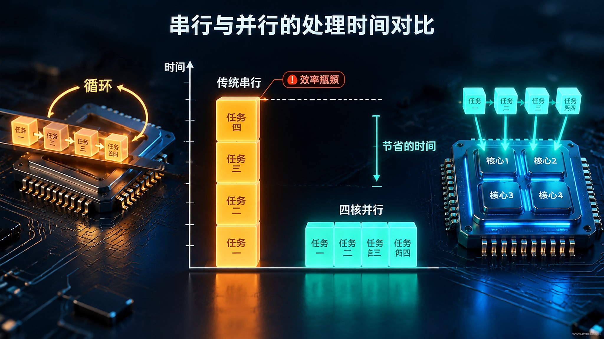
The Efficiency Bottleneck of Traditional Serial CPU Loops

Evolutionary processes depend on population diversity, and diversity means population size and the number of evaluations grow multiplicatively. When candidate evaluations reach the tens of thousands,traditional serial CPU loopsbecome the narrowest segment of the entire pipeline: they process only one individual at a time, leaving the hardware's parallel capability almost entirely idle.

One at a Time: The Execution Model of Serial Loops

The most straightforward implementation treats the entire population as a list and pulls out individuals one by one in a loop: fetch individual → decode into concrete parameters → call the evaluation function → write back the fitness. Adjacent iterations can barely overlap: until the evaluation result returns, the write-back cannot proceed; until the write-back completes, there is nowhere to put the next individual's result. As a result, parallel units such as multi-core CPUs, SIMD, and GPUs sit idle most of the time, watching a single individual run through the pipeline.

Where Does the Overhead Actually Come From?

Linearly ballooning evaluation counts: total evaluations are roughly population size × number of generations. At the 10⁵ scale, serial wall-clock time grows approximately linearly.
Interpreter-level one-by-one execution: per-individual looping, bounds checking, and type dispatch introduce a fixed yet substantial constant overhead.
Non-contiguous memory access and data movement: individuals fetched one by one are often non-contiguous in memory, resulting in low cache hit rates and repeatedly incurred transfer costs.
Synchronization and scheduling: to fetch the next individual, the execution flow must repeatedly pause and resume.

Translating Scale into Time

Take a population of 1000 over 100 generations as an example: roughly 100,000 candidate evaluations in total. At an average of 1 ms per evaluation, the evaluation step alone takes about 100 seconds when run serially, and this does not yet include operator computation or scheduling overhead. If restarts are increased from 1 to 5 to maintain diversity, the cost rises approximately linearly to about 500 seconds. For the same workload organized into batches and handed to parallel hardware, wall-clock time is determined mainly by the number of batches rather than the number of individuals.

When Does This Bottleneck Narrow?

Boundary conditions matter just as much: when a single evaluation is extremely cheap (microsecond-level) or the population is very small (fewer than a hundred), scheduling and memory overhead may outweigh computation, the gap between serial and parallel narrows substantially, the marginal benefit of tensorization diminishes, and the bottleneck shifts to scheduling granularity and memory bandwidth. So whether it is worth reworking the execution model must be assessed by weighing evaluation cost together with scale.

A Structural Bottleneck, Not a Code Defect

The efficiency bottleneck of serial CPU loops is at the execution-model level: localized code tuning cannot eliminate it. To truly solve it, you need to refactor one-by-one into batch-by-batch — batching, tensorization, and parallel scheduling — which also becomes the direct motivation for the tensorized computation graph design that follows.

Serial vs. Parallel Time Comparison

With a population of 1000 over 100 generations, there are roughly 100,000 candidate evaluations. At 1 ms per evaluation, serial execution alone takes about 100 seconds for the evaluation step, and 5 restarts raises this approximately linearly to about 500 seconds. Once organized into batches and handed to parallel hardware, wall-clock time is determined mainly by the number of batches rather than the number of individuals.

Question 1

When traditional evolutionary computation evaluates candidate individuals one by one in a serial CPU loop, what is the main execution-model limitation?

It cannot write back or update the population in any form

Adjacent iterations can hardly overlap, leaving parallel units such as multi-core CPUs, SIMD, and GPUs idle most of the time

It can only handle binary-encoded individual representations

It cannot define a fitness function and therefore cannot evaluate any candidate individual

Question 2

With a population size of 1000 over 100 generations and an average of 1 ms per candidate evaluation, approximately how much wall-clock time does the evaluation step alone take under serial execution?

About 100 seconds

About 1 second

About 10 seconds

About 10,000 seconds

Question 3

Which of the following is NOT a factor that amplifies the constant overhead of serial loops?

Per-individual interpreter-level looping

Per-individual bounds checking and type dispatch

Tensorized batch scheduling

Non-contiguous memory access and frequent data movement

Question 4

Under a batch-parallel execution model, what mainly determines the wall-clock time to complete the same total workload (e.g., 10⁵ evaluations)?

The number of batches and the time per batch

The total number of candidate individuals

The length of the population encoding

The value of the random seed

Question 5

In which of the following situations is judging a serial loop to be a structural bottleneck most likely to be unwarranted?

Multiple independent restarts are needed to maintain diversity

A single evaluation drops to microsecond level, and the population size is only on the order of a hundred

The evaluation function involves an expensive high-precision physical simulation

Each evaluation takes millisecond-level time, and the population scales into the tens of thousands

Case Study: Choosing an Execution Model for 100,000 Evaluations

Read the scenario and answer the questions in light of the efficiency bottleneck of serial loops.

A team is using an evolutionary algorithm to optimize a set of engineering parameters: population size 1000, 100 generations, and each candidate individual's evaluation calls a simulation that averages 1 ms. The current implementation is a traditional serial CPU loop that performs decoding, evaluation, and write-back one by one. The team wants to cut each experimental run from over ten minutes down to the minute level without sacrificing solution quality; at the same time, to maintain population diversity, they plan to increase the number of independent restarts from 1 to 5.

Estimate the wall-clock time of the evaluation step alone in the current serial implementation, and explain how it changes when the number of restarts is increased from 1 to 5. Based on this, determine where the optimization effort should focus.

Answer:
A single run involves about 1000 × 100 = 10⁵ candidate evaluations, which at 1 ms each amounts to about 100 seconds; with 5 restarts, that becomes about 5 × 10⁵ evaluations, or roughly 500 seconds, with wall-clock time ballooning near-linearly. This shows that constant-factor tweaks inside operators yield limited gains; the optimization focus should be at the execution-model level — batching, tensorization, and parallel scheduling — so that wall-clock time is determined by the number of batches rather than the number of individuals.

If the team switches to a batch-parallel execution model, what boundary conditions should also be considered to judge whether this rework is worth it? Give at least two and explain how they affect the payoff.

Answer:
First, evaluation cost and scale: if a single evaluation drops to microsecond level, or the population shrinks below a hundred, scheduling and memory-movement overhead may outweigh computation, and the parallel payoff diminishes. Second, constraints on the number of batches and batch size: batch size is limited by GPU memory and memory bandwidth as well as per-batch computation time, and overly large batches raise per-batch latency and synchronization costs. Third, data layout and memory access: if candidate individuals cannot be organized into contiguous, vectorizable tensors, batch processing still suffers from non-contiguous memory access. Overall, reworking the execution model pays off significantly only when both the number of evaluations and the per-evaluation cost are large enough.