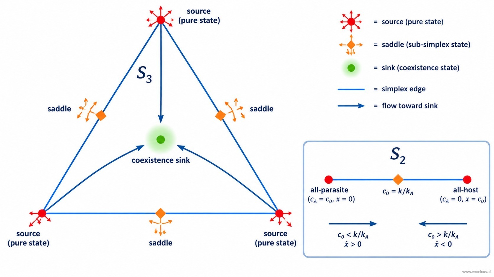
In constant-organization hypercycle and selection models, the state space for concentrations is the invariant concentration simplex = {xᵢ ≥ 0, Σᵢ xᵢ = c0} (or the normalized version with Σᵢ xᵢ = 1). A fixed point is a stationary concentration distribution satisfying ẋᵢ = 0 for , 2, ..., n. At such a point, production/amplification exactly balances decomposition, dilution, and outflow for every species. Fixed-point analysis in the simplex compares selective outcomes by locating stationary states and then classifying their stability: corners and faces correspond to pure or reduced states, interior points represent coexistence, and each point can be a sink, saddle, or source.
Boundary faces are invariant whenever absent species remain absent: if xᵢ = 0, the dynamics preserves xᵢ = 0. A corner of is therefore a pure fixed point in which one species or linked unit dominates; in hypercyclic systems such corners often represent collapsed or non-hypercyclic outcomes. Edge and face fixed points are fixed points of sub-simplices, with only a subset of species present. They are essential for analyzing selection among subsets and for testing invasion by missing members. An interior fixed point has all n members positive and represents coexistence; for a hypercycle, the symmetric interior point is the candidate coherent state.
Stability and Selective Outcome
A fixed point alone does not determine the outcome. Local stability requires linearization: the Jacobian matrix J with entries Jᵢⱼ = ∂ẋᵢ/∂xⱼ evaluated at the fixed point. The eigenvalues of J (restricted to the simplex tangent space) classify the point as a sink (all relevant eigenvalues negative: nearby trajectories converge), a source (all relevant eigenvalues positive: trajectories diverge), or a saddle (some directions attract, others repel). Global outcome also depends on basins of attraction and on the flow along the boundaries. Comparing fixed points by stability and basin size predicts whether the system shows exclusion, partial coexistence, or full hypercyclic persistence.
For a two-component parasite–host system in S2, the equations are
, , .
The system has two corner fixed points in S2: the all-parasite state (, ) and the all-host state (, ). Linearization near the parasite background gives a threshold at : the host concentration satisfies when and when . Thus the ratio of total concentration to the rate ratio decides whether the missing host can invade the parasite state or whether the parasite state repels it. This is the simplest example of how fixed-point analysis converts local rate balances into a global selective prediction.
Key Distinction
A fixed point is stationary by definition, but only stability analysis in the simplex tangent space tells you whether it acts as a sink, saddle, or source. Always combine ẋᵢ = 0 with the Jacobian before drawing conclusions about selection.
Fixed-Point Analysis in the Concentration Simplex
The concentration simplex S 3 is drawn as a triangle. Corners represent pure-state fixed points, edge fixed points represent sub-simplex states, and the interior fixed point is the candidate coexistence sink. The inset S 2 edge shows the parasite–host corner fixed points and the threshold c /kA that reverses the host growth direction.
QUESTION 1
In a constant-organization model on the concentration simplex , what exactly does the fixed-point condition ẋᵢ = 0 for all i state?
The Jacobian matrix has no eigenvalues.
Every species has zero concentration.
The total concentration c0 is zero.
Amplification/production exactly balances decomposition, dilution, and outflow for every species.
✅ Correct!
At a fixed point each species' net rate vanishes, so the concentration distribution is stationary.
❌ Incorrect
Recall that ẋᵢ is the net rate of change of species i; setting it to zero means all gain and loss terms cancel per species.
QUESTION 2
In the concentration simplex , what does a corner (vertex) fixed point represent?
A sub-simplex in which only n−1 species persist.
Full coexistence of all n species.
A saddle point that always attracts interior trajectories.
A pure state where one species or linked unit dominates.
✅ Correct!
Corners are boundary fixed points with xᵢ = c0 for one species and zero for the rest; in hypercyclic systems they often correspond to collapsed or non-hypercyclic outcomes.
❌ Incorrect
A corner lies on the boundary of the simplex, so it cannot have all species positive.
QUESTION 3
Consider the two-component parasite–host system in S2 with ċA = kA cA² − (cA/c0)(kA cA² + k cA x) and cA x − (x/c0)(kA cA² + k cA x). If the system is in the parasite background and /kA, what happens to the host concentration x?
x grows .
x oscillates without changing its average.
x decays .
x remains exactly constant for all initial values.
✅ Correct!
Linearization near the parasite corner gives when /kA, so the missing host can grow in the parasite background.
❌ Incorrect
The threshold /kA reverses the sign of ẋ; below the threshold the host concentration increases.
QUESTION 4
How is a saddle fixed point classified in a local stability analysis?
It has no eigenvalues, so linearization is impossible.
It attracts trajectories from all nearby directions.
It repels trajectories in all nearby directions.
It attracts along some directions and repels along others.
✅ Correct!
A saddle has both stable and unstable directions in the tangent space of the simplex.
❌ Incorrect
Sinks attract in all relevant directions, sources repel in all relevant directions, and saddles mix the two.
QUESTION 5
Why is solving ẋᵢ = 0 alone not enough to predict the selective outcome?
Because total concentration c0 is always zero.
Because the simplex has no boundary.
Because fixed points never exist in hypercycle models.
Because local stability and basins of attraction require Jacobian/linearization and boundary-flow analysis.
✅ Correct!
The selective outcome depends on which fixed point attracts typical initial conditions; this requires stability classification and basin analysis, not just stationary conditions.
❌ Incorrect
Stationary points must still be classified as sinks, saddles, or sources, and their basins determine the actual outcome.
Case Study: Threshold Selection in a Two-Member Simplex
Use fixed-point analysis on S2 to interpret the parasite–host threshold.
A two-component system in constant organization has total concentration c0 = cA + x. The parasite A is autocatalytic with rate kA cA², while the host x has rate k cA x. The rate equations are ċA = kA cA² − (cA/c0)(kA cA² + k cA x), cA x − (x/c0)(kA cA² + k cA x). The simplex S2 is the line segment cA ≥ 0, , cA + . The system has two corner fixed points. You are asked to interpret them and determine the threshold that decides whether the host can invade the parasite background.
Q
Identify the two corner fixed points of S2 for this system and interpret each one biologically.
Answer: The corner fixed points are (cA = c0, ), the all-parasite state, and (cA = 0, ), the all-host state. At each corner the absent species has zero concentration and its rate is zero, so the state is stationary. Biologically they correspond to pure outcomes: either the parasite dominates and the host is absent, or the host dominates and the parasite is absent. In a hypercyclic interpretation these corners are non-coexistent, collapsed states.
Q
State the threshold condition that determines whether the host concentration x grows or decays when the system is near the all-parasite corner. What does this imply for the selective outcome as c0 varies?
Answer: The threshold condition is /kA. Below it, so the host grows in the parasite background; above it, so the host decays. Thus for /kA the all-parasite corner is unstable to host invasion, while for /kA the all-parasite corner is locally attracting and the host cannot invade. The selective outcome therefore changes from host invasion or coexistence to parasite exclusion as c0 crosses k/kA.
which leads to for and for . (2) The parasite is self-reproductive (Fig. 43b): ( x), ( x) (T.13.8) The system has two fixed points at the corners of :