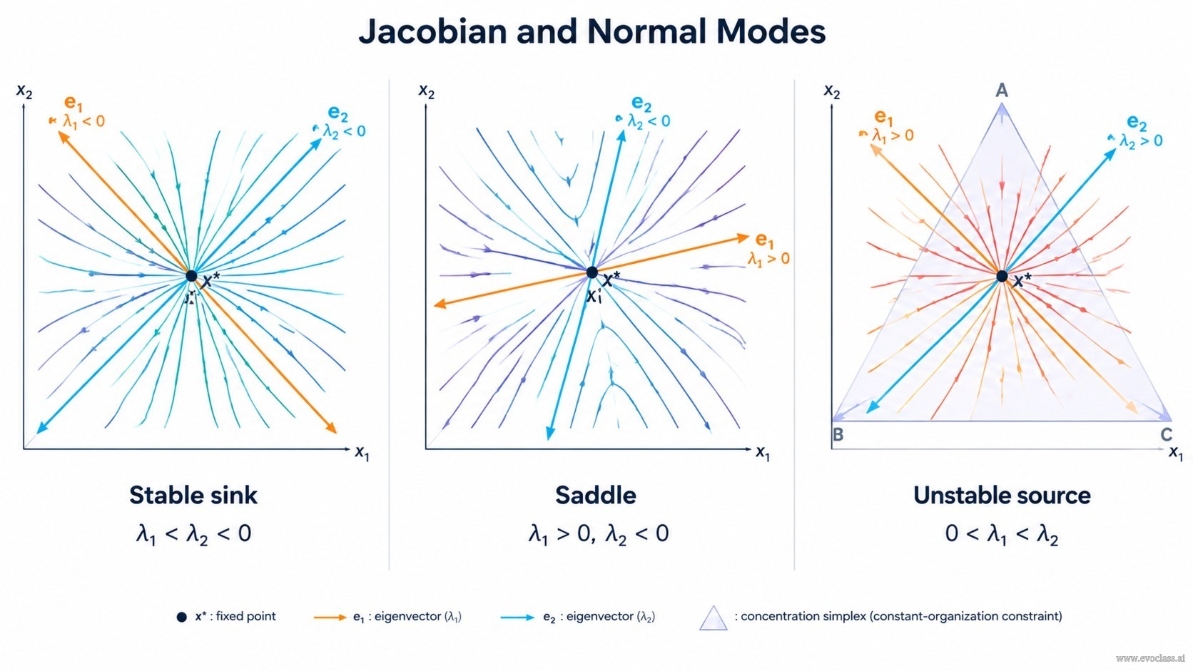
Normal-Mode Linearization and the Jacobian

Near a fixed point x* where F(x*) = 0, the dynamics of a nonlinear system δẋ = F(x*) + J δx + ... can be approximated by its first-order Taylor expansion: δẋ = J(x*) δx. The Jacobian matrix J has entries J_ij = ∂/∂ evaluated at x*. This linearization is valid only for sufficiently small perturbations δx and a nondegenerate Jacobian (det ).

Jacobian and Normal Modes

The eigenvalues and eigenvectors of J define the normal modes. If J is diagonalizable, an affine transformation δx = P y decouples the linearized equations into ẏ_i = , where P is the matrix of eigenvectors. Each mode evolves exponentially as e^{λ_i t}.

'How to carry out this new subdivision is suggested by the structure of the differential equations (6). It corresponds actually to an affine transformation of the x-coordinate system, well known from the theory of linear differential equations. One obtains a new set of equations for the transformed population variables y_i which reads:'

Stability Classification

Re for all i ⇒ asymptotically stable sink (node or focus).
Re for some i ⇒ unstable source or saddle; if mixed signs, saddle.
Zero or purely imaginary eigenvalues ⇒ marginal case; nonlinear or constrained analysis required.

Degenerate Cases and Simplex Constraints

If J is not diagonalizable, Jordan blocks produce polynomial-in-t factors multiplying exponentials. Under constant organization, the dynamics lies on the concentration simplex Σx_i = constant. One mode may be neutral or normalization-related, so stability should be assessed on the tangent or reduced subspace. Normal coordinates make the structure explicit.

Limitations

Linearization predicts only local behavior. It does not determine global stability, limit cycles, Hopf bifurcations, heteroclinic cycles, or invasion outcomes far from the fixed point.

Jacobian and Normal Modes

Three phase portraits illustrating local linearization: stable sink with inward trajectories, saddle with mixed directions, and unstable source with outward trajectories. Eigenvector axes are labeled with eigenvalues λ 1 and λ 2, marking the local neighborhood around the fixed point x*.

QUESTION 1

In normal-mode linearization, what is the primary purpose of the affine transformation δx = P y when the Jacobian is diagonalizable?

To decouple the linearized equations into independent normal modes ẏ_i =

To map the fixed point to infinity.

To eliminate all nonlinear terms.

To rotate the coordinate system so the Jacobian becomes symmetric.

QUESTION 2

For a two-variable system with rate functions F₁(

) and F₂(

), the Jacobian matrix at fixed point x* is:

[[∂F₁/∂

, ∂F₁/∂

], [∂F₂/∂

, ∂F₂/∂

]] evaluated at x*.

[[∂²F₁/∂

, ∂²F₁/∂

], [∂²F₂/∂

, ∂²F₂/∂

]] evaluated at x*.

The inverse of the Hessian matrix of F.

[[F₁, F₂], [∂F₁/∂

, ∂F₂/∂

]] evaluated at x*.

QUESTION 3

If all eigenvalues of J(x*) have negative real parts, the fixed point is classified as:

a source.

a sink (asymptotically stable).

a saddle.

a center.

QUESTION 4

Which situation cannot be resolved by linearization alone?

Eigenvalues are complex conjugates with negative real part.

One eigenvalue is zero and the Jacobian is non-diagonalizable.

All eigenvalues have positive real parts.

All eigenvalues have negative real parts.

QUESTION 5

In a constant-organization system on the concentration simplex Σx_i = constant, why might one eigenvalue of J be zero?

Because the Jacobian is always singular.

Because the system is always unstable.

Because the rate functions are linear.

Because the simplex constraint introduces a neutral mode corresponding to overall normalization.

Case Study: Stability of a Two-Member Hypercycle

Analyze local stability using the Jacobian.

Consider a two-member hypercycle under constant organization. The concentrations

and

satisfy

. The rate equations are

, with the dilution flux

. Let

and

. (a) Find the interior fixed point x*. (b) Compute the Jacobian J at x* and determine its eigenvalues. (c) Classify the stability of x* and describe the local behavior of small perturbations.

Find the interior fixed point x* for

, and compute the Jacobian matrix J at x*. Show your derivation of the partial derivatives.

Answer:
Fixed point: set

. For

, we need

and

. Thus

. With

, solve

. The dilution flux is Φ* =

. The Jacobian entries: ∂F₁/∂

= -2/3; ∂F₁/∂

; ∂F₂/∂

= -2/3. So J = [[-2/3, 0], [0, -2/3]].

Determine the eigenvalues of J, classify the stability of x*, and describe the local behavior of small perturbations.

Answer:
The eigenvalues are

= -2/3 (both negative real). Thus the fixed point is an asymptotically stable sink. Because J = (-2/3) I is a scalar multiple of the identity, the eigenspace is two-dimensional: every direction is an eigenvector, so small perturbations decay isotropically as e^{-2t/3}. The fixed point is a stable star node, and the system returns to x* without oscillation.